Project Goal and Deliverables
The project was built to answer three business questions regarding customer retention: what is happening in the customer base now, why is it happening, and what can we do to improve the future? To answer that, I built an end-to-end workflow starting with raw telecom customer data, loading and cleaning it in SQL Server (SSMS), building an interactive Power BI dashboard, and finally training a machine-learning model to predict future churn.
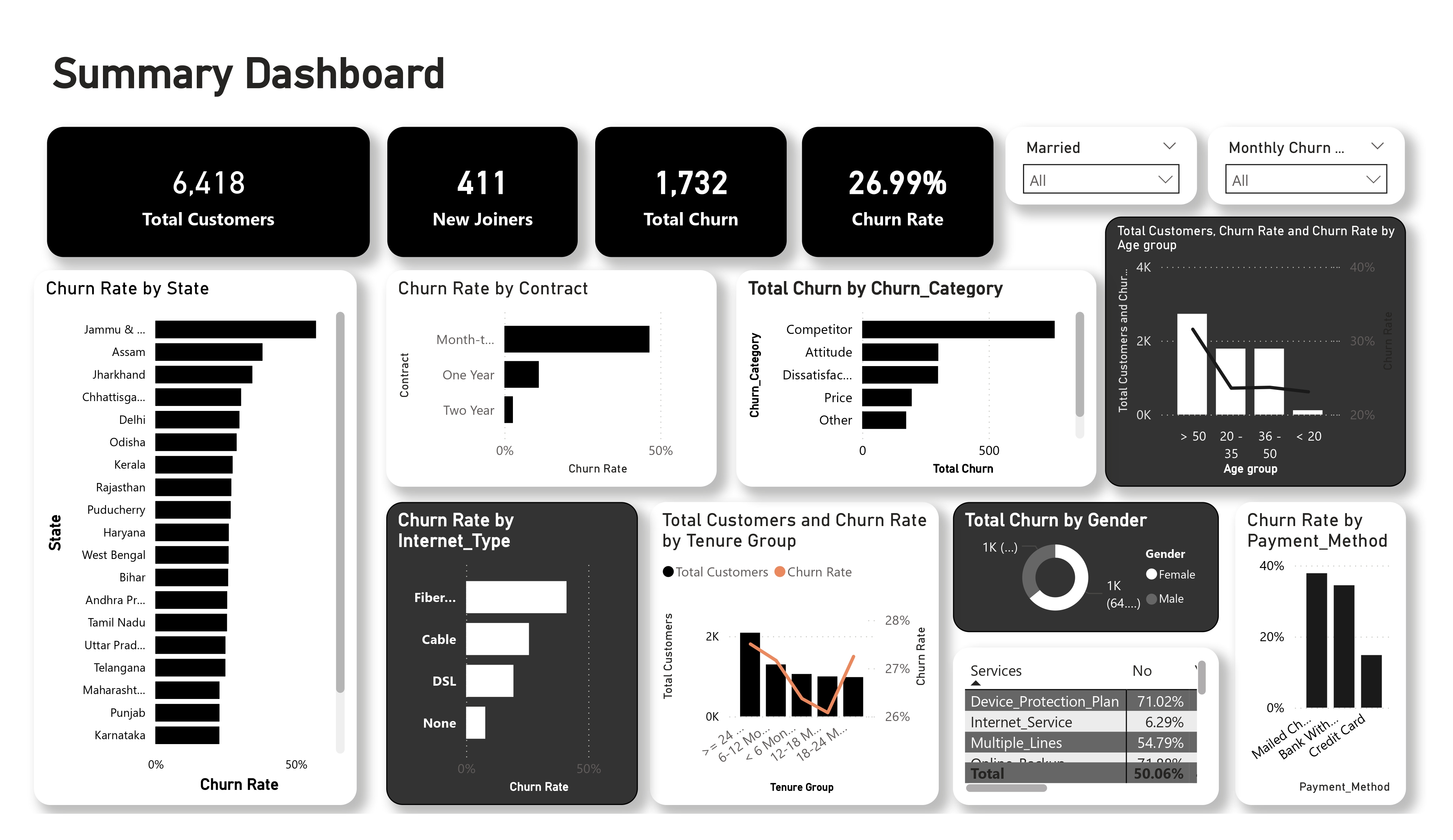
Real-time visibility into the customer base.
Identifying why customers are leaving.
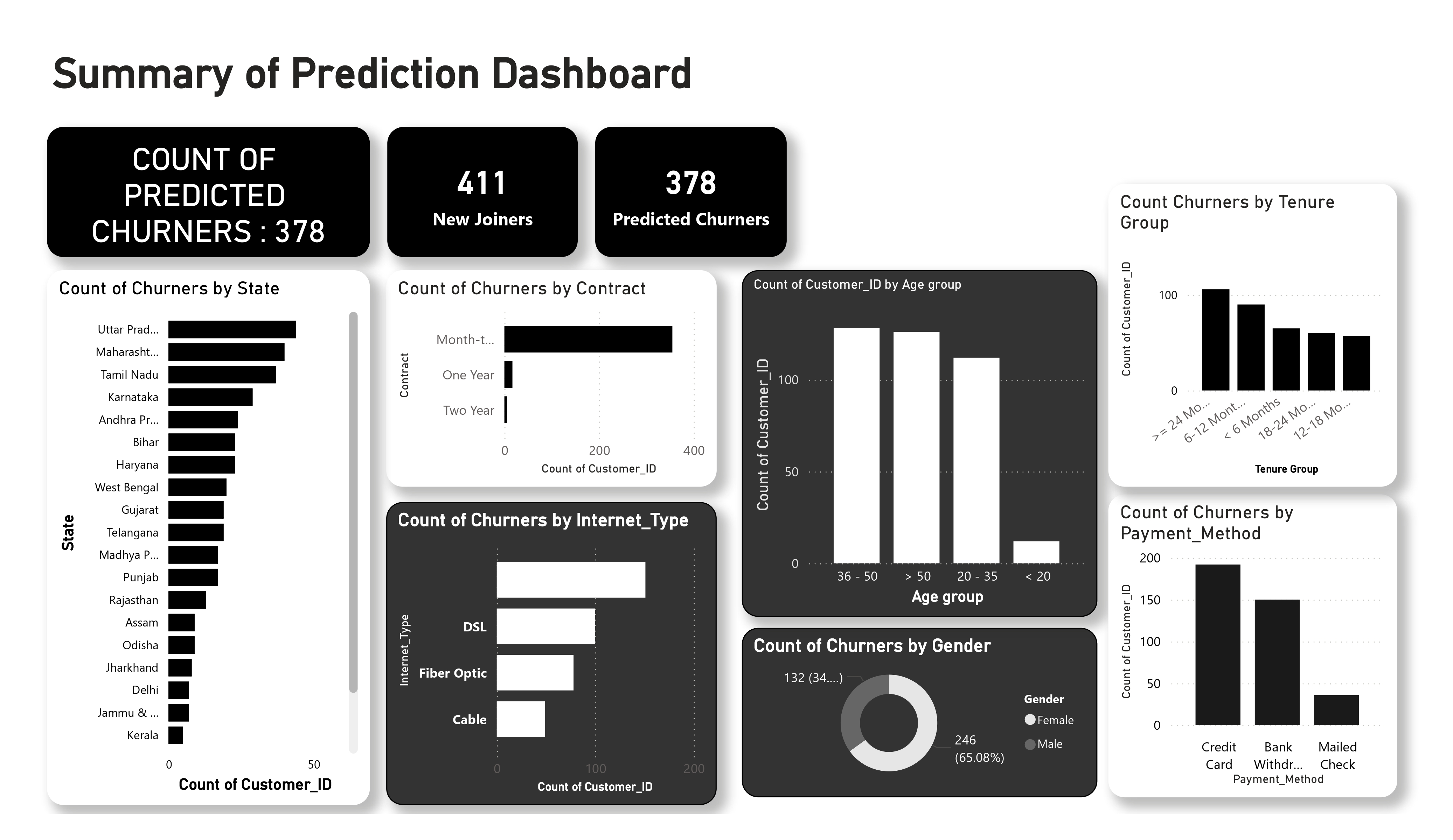
Scoring at-risk customers for retention.
- Main business goals: reduce churn rate, identify high-risk demographics, and provide marketing with an actionable list of customers to target.
- Main metrics used throughout the project: total customers, new joiners, churn rate, and churn status.
- Final outputs: a historical churn dashboard, a predictive churn dashboard, and a CSV export of high-risk customers for the marketing team.
The final output is an end-to-end workflow: raw data cleaning in SQL Server (SSMS), interactive visualization in Power BI, and predictive modeling using Python.
Dataset Engineering
Understanding the Source Data
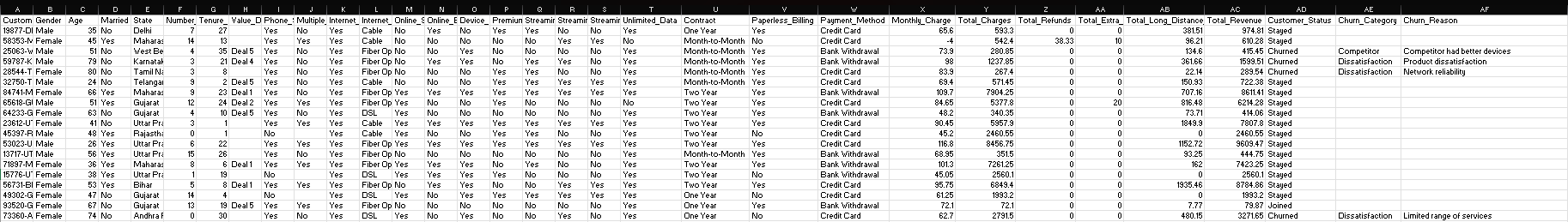
The dataset used in this project is telecom customer churn data. Each row represents a unique customer, identified by Customer_ID. The features cover demographics, geography, referrals, service subscriptions, and revenue metrics. The remaining columns include various categorical and numeric fields such as gender, age, state, contract type, and revenue totals, but the most important field for this project is Customer_Status.
The central business metric. Indicates whether the customer Stayed, Churned, or Joined. This field drives both the historical analysis and the ML target labels.
Provides the high-level reason for departure (Competitor, Dissatisfaction, Price, etc.), allowing for thematic grouping of customer feedback and behavior.
- Customer_Status: either Stayed (still a customer), Churned (left the company), or Joined (new customer). This is the label being explored and predicted.
- Churn_Category: the broad reason why the customer left.
- Churn_Reason: the specific detail behind the category.
df = pd.read_excel(file_path, sheet_name=sheet_name)

print("=" * 50)
print("DATASET OVERVIEW")
print("=" * 50)

print("Shape of dataset:", df.shape)
print("\nColumns:")
print(df.columns.tolist())

print("\nData types:")
print(df.dtypes)

print("\nFirst 5 rows:")
print(df.head())

print("\nLast 5 rows:")
print(df.tail())

print("\nMissing values:")
print(df.isnull().sum())

print("\nDuplicate rows:")
print(df.duplicated().sum())

print("\nUnique values per column:")
print(df.nunique())

print("\nStatistical summary:")
print(df.describe(include="all"))==================================================
DATASET OVERVIEW
==================================================
Shape of dataset: (6007, 32)
Columns:
['Customer_ID', 'Gender', 'Age', 'Married', 'State', 'Number_of_Referrals', 'Tenure_in_Months', 'Value_Deal', 'Phone_Service', 'Multiple_Lines', 'Internet_Service', 'Internet_Type', 'Online_Security', 'Online_Backup', 'Device_Protection_Plan', 'Premium_Support', 'Streaming_TV', 'Streaming_Movies', 'Streaming_Music', 'Unlimited_Data', 'Contract', 'Paperless_Billing', 'Payment_Method', 'Monthly_Charge', 'Total_Charges', 'Total_Refunds', 'Total_Extra_Data_Charges', 'Total_Long_Distance_Charges', 'Total_Revenue', 'Customer_Status', 'Churn_Category', 'Churn_Reason']
Data types:
Customer_ID object
Gender object
Age int64
Married object
State object
Number_of_Referrals int64
Tenure_in_Months int64
Value_Deal object
Phone_Service object
Multiple_Lines object
Internet_Service object
Internet_Type object
Online_Security object
Online_Backup object
Device_Protection_Plan object
Premium_Support object
Streaming_TV object
Streaming_Movies object
Streaming_Music object
Unlimited_Data object
Contract object
Paperless_Billing object
Payment_Method object
Monthly_Charge float64
Total_Charges float64
Total_Refunds float64
Total_Extra_Data_Charges int64
Total_Long_Distance_Charges float64
Total_Revenue float64
Customer_Status object
Churn_Category object
Churn_Reason object
dtype: object
First 5 rows:
Customer_ID Gender Age Married State Number_of_Referrals \
0 11098-MAD Female 30 Yes Madhya Pradesh 0
1 11114-PUN Male 51 No Punjab 5
2 11167-WES Female 43 Yes West Bengal 3
3 11179-MAH Male 35 No Maharashtra 10
4 11180-TAM Male 75 Yes Tamil Nadu 12
Tenure_in_Months Value_Deal Phone_Service Multiple_Lines ... \
0 31 Deal 1 Yes No ...
1 9 Deal 5 Yes No ...
2 28 Deal 1 Yes Yes ...
3 12 NaN Yes No ...
4 27 Deal 2 Yes No ...
Payment_Method Monthly_Charge Total_Charges Total_Refunds \
0 Bank Withdrawal 95.099998 6683.399902 0.00
1 Bank Withdrawal 49.150002 169.050003 0.00
2 Bank Withdrawal 116.050003 8297.500000 42.57
3 Credit Card 84.400002 5969.299805 0.00
4 Credit Card 72.599998 4084.350098 0.00
Total_Extra_Data_Charges Total_Long_Distance_Charges Total_Revenue \
0 0 631.719971 7315.120117
1 10 122.370003 301.420013
2 110 1872.979980 10237.910156
3 0 219.389999 6188.689941
4 140 332.079987 4556.430176
Customer_Status Churn_Category Churn_Reason
0 Stayed Others Others
1 Churned Competitor Competitor had better devices
2 Stayed Others Others
3 Stayed Others Others
4 Stayed Others Others
[5 rows x 32 columns]
Last 5 rows:
Customer_ID Gender Age Married State Number_of_Referrals \
6002 99898-MAH Female 39 No Maharashtra 2
6003 99912-WES Female 60 Yes West Bengal 11
6004 99942-KER Male 59 Yes Kerala 8
6005 99942-TEL Female 34 No Telangana 0
6006 99962-AND Female 63 No Andhra Pradesh 7
Tenure_in_Months Value_Deal Phone_Service Multiple_Lines ... \
6002 14 NaN Yes Yes ...
6003 26 Deal 4 Yes No ...
6004 18 NaN Yes No ...
6005 34 NaN Yes Yes ...
6006 1 Deal 2 Yes Yes ...
Payment_Method Monthly_Charge Total_Charges Total_Refunds \
6002 Bank Withdrawal 65.199997 3687.850098 0.0
6003 Bank Withdrawal 19.650000 244.800003 0.0
6004 Bank Withdrawal 69.699997 69.699997 0.0
6005 Credit Card 70.900002 4677.100098 0.0
6006 Credit Card 91.599998 4627.799805 0.0
Total_Extra_Data_Charges Total_Long_Distance_Charges Total_Revenue \
6002 0 87.779999 3775.629883
6003 0 430.690002 675.489990
6004 0 21.520000 91.220001
6005 0 1880.020020 6557.120117
6006 60 937.039978 5624.839844
Customer_Status Churn_Category Churn_Reason
6002 Stayed Others Others
6003 Stayed Others Others
6004 Churned Attitude Attitude of service provider
6005 Stayed Others Others
6006 Stayed Others Others
[5 rows x 32 columns]
Missing values:
Customer_ID 0
Gender 0
Age 0
Married 0
State 0
Number_of_Referrals 0
Tenure_in_Months 0
Value_Deal 3297
Phone_Service 0
Multiple_Lines 0
Internet_Service 0
Internet_Type 1223
Online_Security 0
Online_Backup 0
Device_Protection_Plan 0
Premium_Support 0
Streaming_TV 0
Streaming_Movies 0
Streaming_Music 0
Unlimited_Data 0
Contract 0
Paperless_Billing 0
Payment_Method 0
Monthly_Charge 0
Total_Charges 0
Total_Refunds 0
Total_Extra_Data_Charges 0
Total_Long_Distance_Charges 0
Total_Revenue 0
Customer_Status 0
Churn_Category 0
Churn_Reason 0
dtype: int64
Duplicate rows:
0
Unique values per column:
Customer_ID 6007
Gender 2
Age 67
Married 2
State 22
Number_of_Referrals 16
Tenure_in_Months 36
Value_Deal 5
Phone_Service 2
Multiple_Lines 2
Internet_Service 2
Internet_Type 3
Online_Security 2
Online_Backup 2
Device_Protection_Plan 2
Premium_Support 2
Streaming_TV 2
Streaming_Movies 2
Streaming_Music 2
Unlimited_Data 2
Contract 3
Paperless_Billing 2
Payment_Method 3
Monthly_Charge 1543
Total_Charges 5756
Total_Refunds 442
Total_Extra_Data_Charges 16
Total_Long_Distance_Charges 5219
Total_Revenue 5974
Customer_Status 2
Churn_Category 6
Churn_Reason 21
dtype: int64
Statistical summary:
Customer_ID Gender Age Married State \
count 6007 6007 6007.000000 6007 6007
unique 6007 2 NaN 2 22
top 11098-MAD Female NaN No Uttar Pradesh
freq 1 3779 NaN 3012 581
mean NaN NaN 47.289163 NaN NaN
std NaN NaN 16.805110 NaN NaN
min NaN NaN 18.000000 NaN NaN
25% NaN NaN 33.000000 NaN NaN
50% NaN NaN 47.000000 NaN NaN
75% NaN NaN 60.000000 NaN NaN
max NaN NaN 84.000000 NaN NaN
Number_of_Referrals Tenure_in_Months Value_Deal Phone_Service \
count 6007.000000 6007.00000 2710 6007
unique NaN NaN 5 2
top NaN NaN Deal 2 Yes
freq NaN NaN 758 5417
mean 7.439820 17.39454 NaN NaN
std 4.622369 10.59292 NaN NaN
min 0.000000 1.00000 NaN NaN
25% 3.000000 8.00000 NaN NaN
50% 7.000000 17.00000 NaN NaN
75% 11.000000 27.00000 NaN NaN
max 15.000000 36.00000 NaN NaN
Multiple_Lines ... Payment_Method Monthly_Charge Total_Charges \
count 6007 ... 6007 6007.000000 6007.000000
unique 2 ... 3 NaN NaN
top No ... Bank Withdrawal NaN NaN
freq 3335 ... 3415 NaN NaN
mean NaN ... NaN 65.087598 2430.986173
std NaN ... NaN 31.067808 2267.481295
min NaN ... NaN -10.000000 19.100000
25% NaN ... NaN 35.950001 539.949982
50% NaN ... NaN 71.099998 1556.849976
75% NaN ... NaN 90.449997 4013.900024
max NaN ... NaN 118.750000 8684.799805
Total_Refunds Total_Extra_Data_Charges Total_Long_Distance_Charges \
count 6007.000000 6007.000000 6007.000000
unique NaN NaN NaN
top NaN NaN NaN
freq NaN NaN NaN
mean 2.038612 7.015149 797.283311
std 8.065520 25.405737 854.858840
min 0.000000 0.000000 0.000000
25% 0.000000 0.000000 107.084999
50% 0.000000 0.000000 470.220001
75% 0.000000 0.000000 1269.839966
max 49.790001 150.000000 3564.719971
Total_Revenue Customer_Status Churn_Category Churn_Reason
count 6007.000000 6007 6007 6007
unique NaN 2 6 21
top NaN Stayed Others Others
freq NaN 4275 4275 4275
mean 3233.246020 NaN NaN NaN
std 2856.181081 NaN NaN NaN
min 21.610001 NaN NaN NaN
25% 833.684998 NaN NaN NaN
50% 2367.149902 NaN NaN NaN
75% 5105.685059 NaN NaN NaN
max 11979.339844 NaN NaN NaN
[11 rows x 32 columns]Processes
SQL Data Orchestration
Load the Raw Data into SQL Server
A relational database provides the robustness needed for repeatable ETL processes. I initialized the db_customersegmentation environment to serve as the unified storage layer.
Staging Layer Implementation
Raw files are first ingested into a stg_customersegmentation table. This isolation ensures that the source data remains untouched while we perform transformations in the production layer.
- • Primary Key enforcement on Customer_ID
- • VARCHAR migration for BIT types
[ Why these choices were made ]
- SQL Server is more powerful for data exploration and cleaning than Excel, especially when the file size increases.
- It allows for repeatable logic. I can run the same cleaning script again if the raw data is updated.
- A database is a better source for Power BI than a local file when working in a professional BI workflow.
SELECT Gender, Count(Gender) as TotalCount,
Count(Gender) * 1.0 / (Select Count(*) from stg_customersegmentation)  as Percentage
from stg_customersegmentation
Group by Gender

SELECT Contract, Count(Contract) as TotalCount,
Count(Contract) * 1.0 / (Select Count(*) from stg_customersegmentation)  as Percentage
from stg_customersegmentation
Group by Contract

SELECT Customer_Status, Count(Customer_Status) as TotalCount, Sum(Total_Revenue) as TotalRev,
Sum(Total_Revenue) / (Select sum(Total_Revenue) from stg_customersegmentation) * 100  as RevPercentage
from stg_customersegmentation
Group by Customer_Status

SELECT State, Count(State) as TotalCount,
Count(State) * 1.0 / (Select Count(*) from stg_customersegmentation)  as Percentage
from stg_customersegmentation
Group by State
Order by Percentage desc
Before cleaning, it is important to understand the data distribution. I used SQL to check:
- the total count and percentage of customers by gender.
- the distribution of customers across different contract types.
- the total revenue coming from each customer status (Stayed, Churned, Joined).
- the states with the highest number of customers.
- any columns with null values that need cleaning later.
Data Cleansing
The transition from stg to prod involves rigorous null-handling and data standardization. Blanks are replaced with logical placeholders (e.g., "None", "Others") to prevent reporting errors.
[ Why this cleaning step matters ]
- Blanks can break grouping and filtering, especially in dashboards.
- Readable replacement values make visuals easier to understand than showing blank categories.
- A production table should be the cleaned version that reporting users trust, while the staging table remains the untouched import copy.
SELECT
    Customer_ID, Gender, Age, Married, State, Number_of_Referrals, Tenure_in_Months,
    ISNULL(Value_Deal, 'None') AS Value_Deal,
    Phone_Service,
    ISNULL(Multiple_Lines, 'No') As Multiple_Lines,
    Internet_Service,
    ISNULL(Internet_Type, 'None') AS Internet_Type,
    ISNULL(Online_Security, 'No') AS Online_Security,
    ISNULL(Online_Backup, 'No') AS Online_Backup,
    ISNULL(Device_Protection_Plan, 'No') AS Device_Protection_Plan,
    ISNULL(Premium_Support, 'No') AS Premium_Support,
    ISNULL(Streaming_TV, 'No') AS Streaming_TV,
    ISNULL(Streaming_Movies, 'No') AS Streaming_Movies,
    ISNULL(Streaming_Music, 'No') AS Streaming_Music,
    ISNULL(Unlimited_Data, 'No') AS Unlimited_Data,
    Contract, Paperless_Billing, Payment_Method, Monthly_Charge,
    Total_Charges, Total_Refunds, Total_Extra_Data_Charges,
    Total_Long_Distance_Charges, Total_Revenue, Customer_Status,
    ISNULL(Churn_Category, 'Others') AS Churn_Category,
    ISNULL(Churn_Reason , 'Others') AS Churn_Reason
INTO [db_customersegmentation].[dbo].[prod_customersegmentation]
FROM [db_customersegmentation].[dbo].[stg_customersegmentation];"Clean data is the foundation of trust in any dashboard. By standardizing nulls at the SQL level, we ensure that every filter in Power BI returns accurate, grouped results without 'Blank' artifacts."
Reporting Views
Customer_Status IN ('Churned', 'Stayed'). Used for historical analysis and machine-learning training because these rows already have known outcomes.Customer_Status = 'Joined'. Used later for prediction because these are the customers the model will score as possible future churners.These views become crucial later for prediction. This is because the model needs one dataset with known outcomes for training, and another dataset of newly joined customers for prediction.
Create View vw_customersegmentationData as
select * from prod_customersegmentation where Customer_Status In ('Churned', 'Stayed')

Create View vw_JoinData as
select * from prod_customersegmentation where Customer_Status = 'Joined'Power BI Transformation
Connecting Power BI to the SQL production layer enabled complex Power Query transformations, including numeric churn flagging and charge-bucket categorization.
4.1 Numeric Churn Flag
A custom column named Churn_Status is created in Power Query. If Customer_Status = Churned, the value is 1; otherwise it is 0.
Why this was done: a numeric flag makes it easy to calculate churn totals by simply summing the column. This is much easier than repeatedly filtering text values in every visual.
4.2 Charge Ranges
A custom column for Monthly Charge Status buckets: less than 20, 20 to 50, 50 to 100, and greater than 100.
Why this was done: Monthly Charge has many values. Range buckets make comparisons much easier for business users than using raw detailed numbers.
4.3 Age & Tenure Mapping
Instead of duplicating the full table, I created a Reference table called mapping_AgeGrp. It keeps only the Age column, removes other columns, removes duplicates, and then creates an Age Group column with several bands.
Why Reference was used instead of Duplicate: a duplicate would hit SQL Server again during refresh. A reference reuses the existing query output and is better for model performance.
4.4 Sorting Logic
A Tenure Group Sorting column is added so the x-axis sorts in business order instead of alphabetical order.
Why sorting columns were necessary: Power BI sorts text alphabetically by default. Without helper columns, categories like '12 to 18 months' could appear before '6 to 12 months', which is misleading.
Add a new column in prod_customersegmentation
Churn Status = if [Customer_Status] = "Churned" then 1 else 0
Change Churn Status data type to numbers

Monthly Charge Range = if [Monthly_Charge] < 20 then "< 20" else if [Monthly_Charge] < 50 then "20-50" else if [Monthly_Charge] < 100 then "50-100" else "> 100"Specialized Mapping Tables
4.3 Age Mapping
Instead of duplicating the full table, I created a Reference table called mapping_AgeGrp. It keeps only the Age column, removes other columns, removes duplicates, and then creates an Age Group column with these bands: less than 20, 20 to 35, 35 to 50, and greater than 50.
A separate Age Group Sorting column is then added with numeric values 1 to 4 so that charts display the age groups in logical order.
Keep only Age column and remove duplicates
Age Group = if [Age] < 20 then "< 20" else if [Age] < 36 then "20 - 35" else if [Age] < 51 then "36 - 50" else "> 50"
AgeGrpSorting = if [Age Group] = "< 20" then 1 else if [Age Group] = "20 - 35" then 2 else if [Age Group] = "36 - 50" then 3 else 4
Change data type of AgeGrpSorting
4.4 Tenure Mapping
The same idea is used for Tenure in Months. A reference table called mapping_TenureGrp is created, duplicates are removed, and a Tenure Group column is added with these bands: less than 6 months, 6 to 12 months, 12 to 18 months, 18 to 24 months, and greater than or equal to 24 months.
Keep only Tenure_in_Months and remove duplicates
Tenure Group = if [Tenure_in_Months] < 6 then "< 6 Months" else if [Tenure_in_Months] < 12 then "6-12 Months" else if [Tenure_in_Months] < 18 then "12-18 Months" else if [Tenure_in_Months] < 24 then "18-24 Months" else ">= 24 Months"
TenureGrpSorting = if [Tenure_in_Months] = "< 6 Months" then 1 else if [Tenure_in_Months] =  "6-12 Months" then 2 else if [Tenure_in_Months] = "12-18 Months" then 3 else if [Tenure_in_Months] = "18-24 Months " then 4 else 5
Change data type of TenureGrpSorting
4.5 Service Unpivoting
To analyze many yes/no service columns in one visual, I created another reference table and unpivoted the service fields. This turns many separate columns into two generic fields: Services and Status.
"If every service stayed in its own separate column, a summary visual would be messy. Unpivoting turns the data into a long format that works neatly in a matrix, significantly improving dashboard usability."
Unpivot services columns
Rename Column :
Attribute >> Services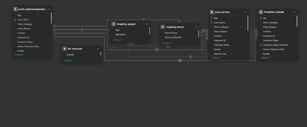
Value >> StatusData Model Schema
Relationships are logically established between the primary production table, mapping tables, and the prediction output table. This clean star-schema layout optimizes filtering and summarization.
Analytical Measures
I developed a suite of DAX measures to drive the dashboard's interactivity. These calculations provide the real-time KPIs necessary for stakeholder decision-making.
Why explicit measures were used instead of relying only on Power BI defaults: explicit measures are reusable, easier to manage, and behave more predictably across visuals and filters.
Total Customers = Count(prod_customersegmentation[Customer_ID])
New Joiners = CALCULATE(COUNT(prod_customersegmentation[Customer_ID]), prod_customersegmentation[Customer_Status] = "Joined")
Total Churn = SUM(prod_customersegmentation[Churn Status])
Churn Rate = [Total Churn] / [Total Customers]Predictive Modeling
Random Forest Classifier
A Random Forest ensemble was chosen for its robustness against over-fitting and its inherent ability to provide feature importance. This model serves as the "brain" of the churn prediction engine.
Pre-processing
Categorical variables were label-encoded, and target leakage was prevented by dropping Churn_Category and Churn_Reason from the training set.
import pandas as pd
import numpy as np
import matplotlib.pyplot as plt
import seaborn as sns
from sklearn.model_selection import train_test_split
from sklearn.ensemble import RandomForestClassifier
from sklearn.metrics import classification_report, confusion_matrix
from sklearn.preprocessing import LabelEncoder
import joblib

# Define the path to the Excel file
file_path = r"C:\Users\User\Documents\Churn Project\Prediction_Data.xlsx"

# Define the sheet name to read data from
sheet_name = 'vw_customersegmentationData'

# Read the data from the specified sheet into a pandas DataFrame
data = pd.read_excel(file_path, sheet_name=sheet_name)

# Display the first few rows of the fetched data
print(data.head())
7.5 Training
A RandomForestClassifier is created with n_estimators = 100. This controls how many decision trees are built; more trees usually make the voting process more stable.
# Initialize the Random Forest Classifier
rf_model = RandomForestClassifier(n_estimators=100, random_state=42)

# Train the model
rf_model.fit(X_train, y_train)The model achieved ~84% accuracy. Feature importance was checked to show which columns the model relies on most, allowing for potential tuning by removing low-importance features.
Confusion Matrix:
[[783  64]
 [126 229]]

Classification Report:
              precision    recall  f1-score   support

           0       0.86      0.92      0.89       847
           1       0.78      0.65      0.71       355

    accuracy                           0.84      1202
   macro avg       0.82      0.78      0.80      1202
weighted avg       0.84      0.84      0.84      1202

[Feature Importance Chart Rendered Successfully]Risk Scoring
The trained model was applied to the Joined cohort, generating churn probabilities for active customers.
- Only rows where
Customer_Status_Predicted = 1are kept for proactive targeting. - Results are exported as a CSV for Power BI integration.
- Customer_ID was retained to identify individual at-risk profiles.
Why Customer_ID had to be kept: The prediction dashboard needs to identify individuals. Without it, connecting prediction output back to custom-level detail would be impossible.
# Define the path to the Joiner Data Excel file
file_path = r"C:\Users\User\Documents\Churn Project\Prediction_Data.xlsx"

# Define the sheet name to read data from
sheet_name = 'vw_JoinData'

# Read the data from the specified sheet into a pandas DataFrame
new_data = pd.read_excel(file_path, sheet_name=sheet_name)

# Display the first few rows of the fetched data
print(new_data.head())

# Retain the original DataFrame to preserve unencoded columns
original_data = new_data.copy()

# Retain the Customer_ID column
customer_ids = new_data['Customer_ID']

# Drop columns that won't be used for prediction in the encoded DataFrame
new_data = new_data.drop(['Customer_ID', 'Customer_Status', 'Churn_Category', 'Churn_Reason'], axis=1)

# Encode categorical variables using the saved label encoders
for column in new_data.select_dtypes(include=['object']).columns:
    new_data[column] = label_encoders[column].transform(new_data[column])

# Make predictions
new_predictions = rf_model.predict(new_data)

# Add predictions to the original DataFrame
original_data['Customer_Status_Predicted'] = new_predictions

# Filter the DataFrame to include only records predicted as "Churned"
original_data = original_data[original_data['Customer_Status_Predicted'] == 1]

# Save the results
original_data.to_csv(r"C:\Users\User\Documents\Churn Project\Prediction_result.csv", index=False)Customer_ID Gender Age Married State Number_of_Referrals \
0 11751-TAM Female 18 No Tamil Nadu 5
1 12056-WES Male 27 No West Bengal 2
2 12136-RAJ Female 25 Yes Rajasthan 2
3 12257-ASS Female 39 No Assam 9
4 12340-DEL Female 51 Yes Delhi 0
Tenure_in_Months Value_Deal Phone_Service Multiple_Lines ... \
0 7 Deal 5 No No ...
1 20 NaN Yes No ...
2 35 NaN Yes No ...
3 1 NaN Yes No ...
4 10 NaN Yes No ...
Payment_Method Monthly_Charge Total_Charges Total_Refunds \
0 Mailed Check 24.299999 38.450001 0.0
1 Bank Withdrawal 90.400002 268.450012 0.0
2 Bank Withdrawal 19.900000 19.900000 0.0
3 Credit Card 19.549999 19.549999 0.0
4 Credit Card 62.799999 62.799999 0.0
Total_Extra_Data_Charges Total_Long_Distance_Charges Total_Revenue \
0 0 0.000000 38.450001
1 0 94.440002 362.890015
2 0 11.830000 31.730000
3 0 10.200000 29.750000
4 0 42.189999 104.989998
Customer_Status Churn_Category Churn_Reason
0 Joined Others Others
1 Joined Others Others
2 Joined Others Others
3 Joined Others Others
4 Joined Others Others
[5 rows x 32 columns]Business Impact & Deliverables
The primary value of this project is that it moves from simple data storage to strategic preparation. By centralising the data in SQL Server and connecting it to a real-time Power BI dashboard, the business gets a single source of truth for its churn metrics.
Marketing teams no longer have to wait until the end of the month to see who left. They can now use the prediction export to find active customers who are likely to leave within the next few weeks and offer them targeted discounts or support.
By identifying that “Competitor” and “Price” are the main churn categories, the business can focus its budget on competitive pricing adjustements rather than on general customer service training.
The automated SQL cleaning pipeline ensures that even if local file errors occur, the production reporting layer remains accurate, reducing the risk of making business decisions on bad or incomplete data.
This project demonstrates how data engineering (SQL), business intelligence (Power BI), and data science (Machine Learning) work together to solve a practical problem. It transforms a historical dataset into a future-facing tool that directly supports business revenue targets.